Measuring color differences in natural scene color images
Here you can find the algorithms (Python files [py-files] and the references [Ref] to the original papers) tested by Ortiz-Jaramillo, et.al. in: B. Ortiz, A. Kumcu and W. Philips, "Evaluating color difference measures in images", International Conference on Quality of Multimedia Experience (QoMEX) 2016. and B. Ortiz, A. Kumcu, L. Platisa and W. Philips, "Evaluation of color differences in natural scene color images", Signal Processing: Image Communication, 2019. Please reference these works if you use any of the code available in this page. To download the files, please navigate to the links in the Table with the state-of-the-art CD measures. For the login information (user name and password) please contact Benhur Ortiz JaramilloAsli.Kumcu@UGent.be indicating the purpose of using this code.
Context
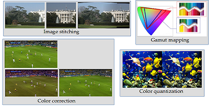
Nowadays, the color-related aspect of image difference assessment has become an active area in the research of color science and imaging technology due to its wide range of applications such as color correction, color quantization, color image similarity and retrieval, image segmentation, gamut mapping, among others. For instance, in multiview imaging, color correction is used to eliminate color inconsistencies between views. Then, the assessment of color corrected images can be used to find the color correction algorithm that produces the smallest difference in terms of color. Color image similarity and retrieval is a process where all images with similar color composition to a query image are retrieved from a database. Thus, the assessment of CDs between images is very important to obtain those images with the minimum perceived CD with respect to the query image. Gamut mapping and color quantization algorithms replace pixel colors following certain criteria to ensure a good correspondence in terms of color between an original image and its reproduction. That is, CD assessment can be used to find the quantization step size and/or the range of displayable colors to obtain the reproduction with the minimum perceived CD. Color image segmentation divides images into regions displaying homogeneous colors. Hence, a CD measure can be used to find the regions with minimum perceived CD between pixels within the same region.
Why do we care about it?
Color differences in natural scene color images
Applications of CD assessment in images
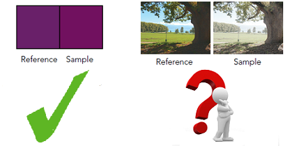
Paired comparison for CD assessment
The most well known and widely used method for comparing two homogeneous color samples is the CIEDE2000 color difference formula because of its strong agreement with human perception. However, the formula is unreliable when applied over images and its spatial extensions have shown little improvement compared with the original formula. Hence, researchers have proposed many methods intending to measure color differences (CDs) in natural scene color images. However, these existing methods have not yet been rigorously compared.
Background
Traditionally, computing CDs in images has been accomplished by using a CD formula on a pixel-by-pixel basis and then examining statistics such as mean, median or maximum. For instance, the CIEDE2000 formula can be used for computing CD in natural scene color images. However, it is well know that the use of this procedure produces big estimation errors because the CIEDE2000 formula was specifically designed for homogeneous color samples. Additionally, there is not standard procedure for computing CDs in images. In search for an adequate solution of this problem, the study of CD measures in natural scene color images is an active area because its wide range of applications such as color correction, color quantization, color image similarity and retrieval, image segmentation, gamut mapping, among others. The most well-known and widely used CD measures for natural scene color images are listed in the following Table. We highly recommend to download the full package located here [Download all measures]
The test data was selected such that the most common applications of the color-related aspect of image difference assessment are included. Particularly, the following applications were considered: color correction, color quantization, color matching, gamut mapping and multiview imaging systems. The test dataset was obtained from three publicly available databases: Tampere Image Database (TID2013), Subject-rated image database for tone-mapped images (SRTMI) and Color quantization database (CQD).
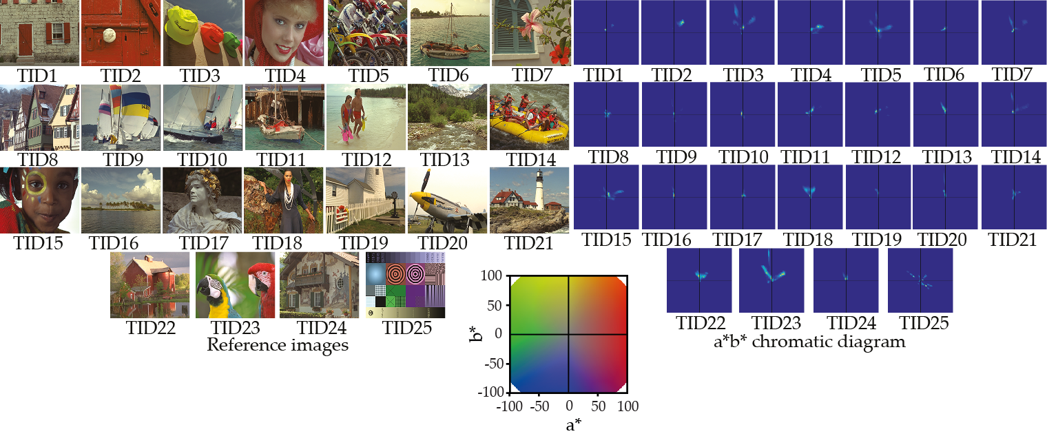
TID2013 contains 25 reference images and 3000 distorted images (25 reference images × 24 types of distortions × 5 levels of distortion).
The 25 source images from the TID2013 database: source images and chromatic histograms (see the chromatic a*b* color chart to identify the color areas of the histograms).
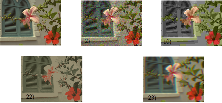
The distortions are (distortions marked in bold produce changes in color): 1) additive Gaussian noise, 2) additive noise in color components, 3) spatially correlated noise, 4) masked noise, 5) high frequency noise, 6) impulse noise, 7) quantization noise, 8) Gaussian blur, 9) image denoising, 10) JPEG compression, 11) JPEG2000 compression, 12) JPEG transmission errors, 13) JPEG2000 transmission errors, 14) non eccentricity pattern noise, 15) local block-wise distortions of different intensity, 16) mean shift (intensity shift), 17) contrast change, 18) change of color saturation, 19) multiplicative Gaussian noise, 20) comfort noise, 21) lossy compression of noisy images, 22) image color quantization with dither, 23) chromatic aberrations, 24) sparse sampling and reconstruction.
Selected set of distortions
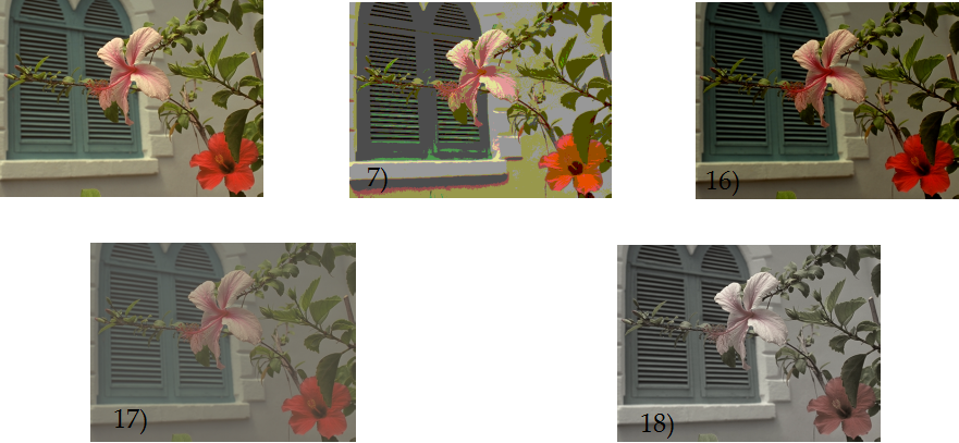
Examples of the discarded data
The following 4 color related distortion types were selected from the 24 types available in TID2013: 7) quantization noise, 16) mean intensity shift, 17) contrast change, and 18) change of color saturation. We selected this subset of distortions because they encompass the most important applications of the color-related aspect of image difference assessment. The remaining 20 distortions were not used because they possess spatial distortions which impact the quality of the image much more strongly than CDs. For instance, we do not use 22) color quantization with dither and 23) chromatic aberrations because even though they have a large influence on color noise, they also produce strong artifacts of spatial nature such as blurring, false edges and/or rainbow edges which impact the quality of the image much more strongly than the CDs.
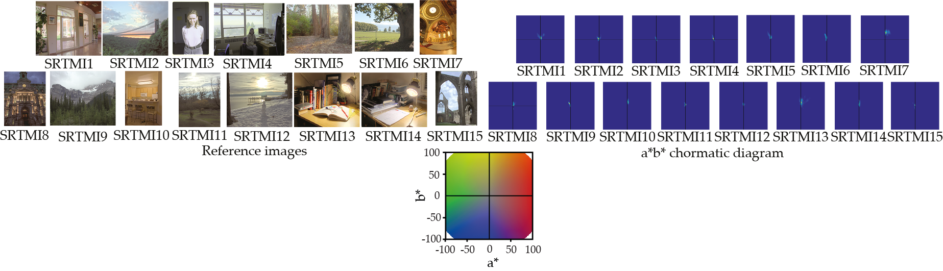
SRTMI contains 15 reference images and 105 distorted images (15 reference images × 7 levels of distortion).
The 15 source images from the SRTMI database: source images and chromatic histograms (see the chromatic a*b* color chart to identify the color areas of the histograms).
In SRTMI database, high dynamic range (HDR) images are converted to low dynamic range (LDR) images. Those images are subjectively evaluated resulting in MOS values of the visual quality of indoors and outdoors HDR images on standard LDR displays. This database provides 15 image sets, each of which contains a HDR image along with 8 tone-mapped images created by color correction and color mapping algorithms. Since differences between HDR and LDR images cannot be assessed directly, we do not use the HDR images and instead we use only the 8 LDR images. Here, the LDR image with the highest MOS per set is considered the reference sample and the other 7 LDR images are the test samples.
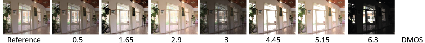
Example of one SRTMI set of images (Reference plus 7 test samples).
The set of images shows the agreement with DMOS (difference between MOS best quality LDR and MOS of the other images) and the image that is closer in terms of CDs to the best quality LDR, i.e., assuming that the best quality LDR image is the reference. Also, it shows that the perceived CDs increase from left to right.
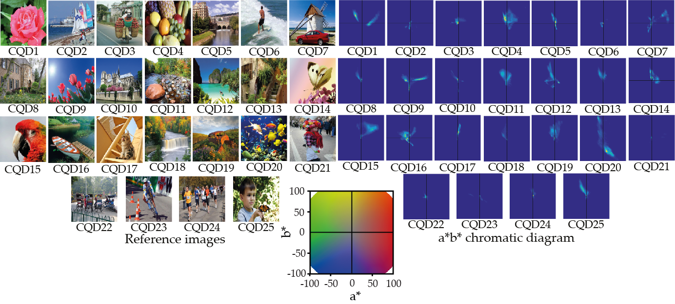
The 25 source images from the CQD database: source images and chromatic histograms (see the chromatic a*b* color chart to identify the color areas of the histograms).
In this database, each of the source images has been quantized with 7 different quantization levels (4, 8, 16, 32, 64, 128, and 256 colors) which differs from the levels used on the TID2013 quantization noise subset (27, 39, 55 and 76 colors). Unlike TID2013 where only the uniform quantization algorithm is used, this database uses five popular color image quantization algorithms: k-means, median cut, Wu's, octree, and Dekker's SOM. These images were evaluated through a subjective quality test in which human subjects were asked to judge the differences between the images resulting in a MOS per processed image. This database increases the diversity of CDs presented in TID2013 database (quantization noise subset) by using different quantization algorithms as well as other quantization levels.
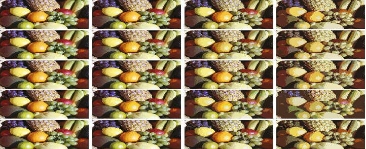
Examples of CDs in CQD. From left to right: (Top) k-means algorithm: reference, mos = 73.52, mos = 33.29, mos = 13.02. (Middle-Top) median cut algorithm: reference, mos = 71.45, mos = 32.09, mos = 14.39. (Middle) Wu's algorithm: reference, mos = 75.45, mos = 33.14, mos = 16.59. (Middle-Bottom) octree algorithm: reference, mos = 56.28, mos = 34.16, mos = 13.65. (Bottom) Dekker's SOM: reference, mos = 71.06, mos = 34.99, mos = 16.98. MOS ranges (0 - min, 100 - max).
The Figure shows one scene from the CQD database and its corresponding quantized images using k-means algorithm (Top), median cut algorithm (Middle-Top), Wu's algorithm (Middle), octree (Middle-Bottom), and Dekker's SOM (Bottom). From left to right reference, 128, 32 and 8 quantization colors. The Figure shows the differences in color presented by the different color quantization algorithms.
Evaluation methodology
The performance of CD measures is evaluated by comparing the predicted CD value to the human scores using various metrics. Particularly, we use Pearson Correlation Coefficient (PCC) and Spearman's Rank Order Correlation Coefficient (SROCC):
For all data: we compute the PCC and the SROCC between the subjective scores and the values computed by the tested CD measures
By type of color related distortion: we compute the PCC and the SROCC between the subjective scores and the CD measure values for each distortion type
By source content: we compute the PCC and the SROCC between the CD measure and the MOS over all distortions and distortion levels for each source image
Also, we use pairwise comparisons as discussed by Garcia et. al.. Here, the related samples are the performances (PCCs and SROCCs) of the CD measures. The objective of the pairwise comparison is to determine if we may conclude from the data (PCCs and SROCCs between CD measures and subjective scores) that there are statistically significant differences in terms of the performance between the benchmark and the other tested CD measures. In addition to the analysis of correlation, we propose a novel methodology to analyse the performance of the CD measures in function of the source image color content.
Content related features
To characterize the image content, we use three color-related features (dominant color, total variance of color and color entropy) and one spatial related feature. The three features related to color describe the color distribution of the image by using a measure of central tendency (dominant color) and two measures of dispersion (total variance and entropy). The spatial activity is a representation of the number of details presented in the image.
Dominant color extraction
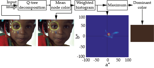
The aforementioned four features are computed as follows: the dominant color [M-File] was computed as the maximum of the color histogram on the CIELAB coordinates (the color histogram is computed using the methology proposed by Ortiz-Jaramillo et.al.). Then it is transformed into the CIELCH (luminance, chroma and hue coordinates) with the purpose of using more intuitive attributes of color for representing the dominant color.
The total variance of color is computed as the trace of the covariance matrix of the CIELAB components, i.e., this is a measure of dispersion of the color information of the image under inspection.
The entropy of the color distribution is computed as a measure of dispersion of the color information as well as a rough estimation of the number of colors within the image (the higher the entropy the wider the color range and more diverse).
For computing the spatial activity of the images, we use the average of the magnitude of SI13 filtered images as proposed by Pinson and Wolf. This is a measure of the spatial activity of the perceived details within the image under analysis.
Results and discussion
For all data and by distortion type
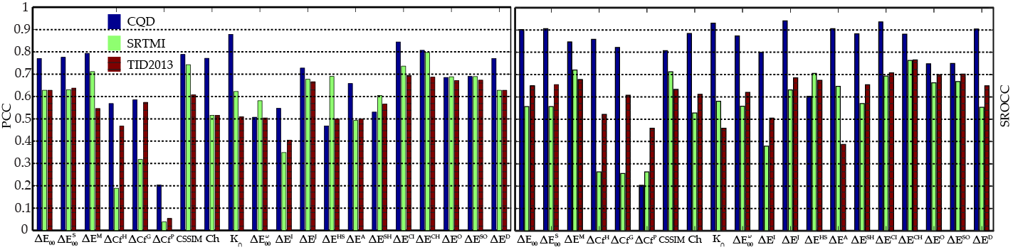
Performance of the considered CD measures for all data and by databases
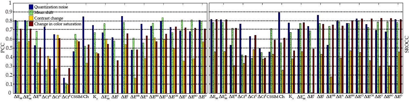
Performance of the considered CD measures for individual distortions on TID2013
Overall the best performing CD measures are Δ ECI and Δ ECH displaying a strong correlation in all tested data. The worst performing methods are Δ EA, Δ EO, Δ ESO, Δ EM, Δ CfH, Δ CfG, Δ CfP, CSSIM, Ch, K∩, Δ EI and Δ EHS displaying a weak correlation. Even though these 12 CD measures perform well in one or two of the subsets, in general, the correlation between these measures and the subjective scores is weak and there are other methods with higher performance. That is, the results suggest that there is not advantage of using such measures in the tested data.
By source content
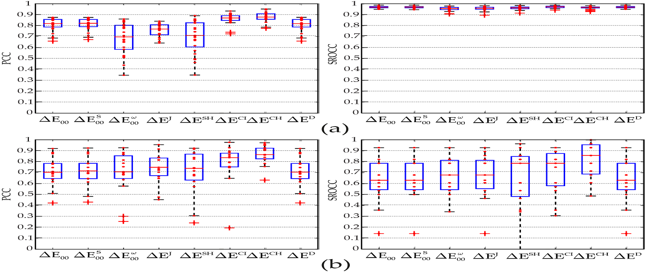
Box plot of the performance of the considered CD measures appraised on (a) CQD and (b) SRTMI per individual source image.
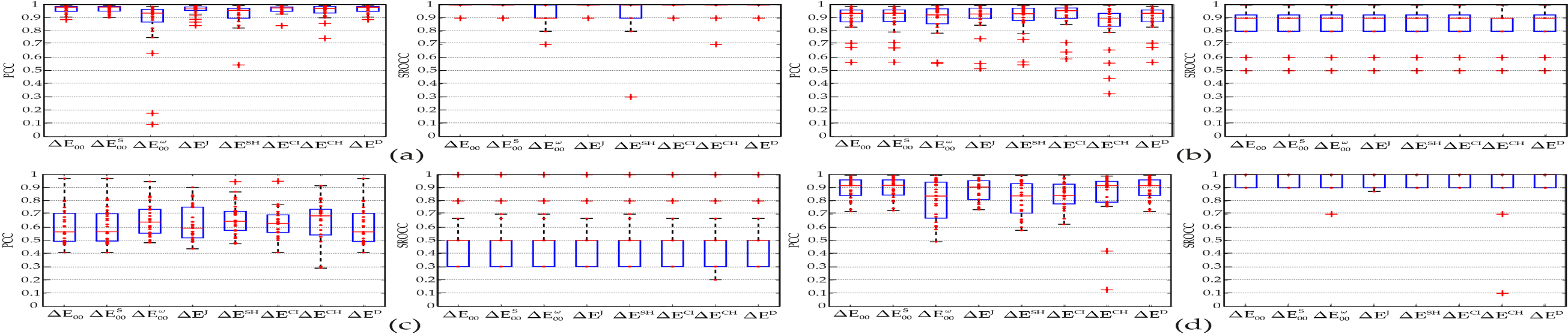
Box plot of the performance of the considered CD measures appraised on (a) quantization noise, (b) mean shift, (c) contrast change and (d) change in color saturation subsets of the TID2013 database per individual source image.
The box plot represents the PCC between the CD measure and the MOS over all distortions and distortion levels for each source image. Thus, it shows the variability of the agreement between the CD measure and the subjective scores for different image content. In summary, the box and bar plots reveal that:
The quantization noise subset is the least challenging type of distortion because the tested CD measures perform considerably well in it compared with their performance in the other tested subsets. Based on the results presented in this work, we found that Δ E00, Δ ES 00, Ch, K∩, Δ EJ, Δ ECI, Δ ECH and Δ ED are the best candidates to be used in color quantization application displaying a strong correlation with subjective scores.
The tested CD measures achieve a strong correlation in the mean shift subset. Based on the results, the best candidates to assess images affected by black level shift are: Δ E00, Δ ES 00, Δ EJ, Δ ECI, Δ ECH and Δ ED.
Because of the variety of color-related distortions in our test data produced by the color mapping algorithms (SRTMI dataset) this distortion appeared the most challenging for assessing CD. Nevertheless, it is still possible to recommend Δ ECI and Δ ECH (showing a moderate correlation with subjective scores) as candidates for assessing CD in color mapped images.
The following CD measures are good candidates for assessing CDs on images affected by change of color saturation: Δ E00, Δ ES 00, Δ EJ, Δ ECI, Δ ECH and Δ ED displaying a moderate correlation with subjective scores.
In the contrast change subset none of the tested CD measures perform well and therefore we recommend to search alternative mechanisms for the assessment of contrast changes in images (cf. Agaian et.al., Panetta et.al. and Ortiz-Jaramillo et.al. for examples).
The data of Figure also shows that there are not significant differences in terms of PCC and SROCC with subjective scores when spatial processing based on filtering is applied prior to computing pixel-wise the CIEDE2000. Specifically, no statistically significant differences exist between Δ E00 and Δ ES 00 (p-value = 0.205). This is mainly because the spatial processing is based on filtering (band pass filtering simulating contrast masking as proposed by Zhang and Wandell), relying on the computation of pixel-wise differences between the images, and the use of the average as the overall CD.
Color content analysis
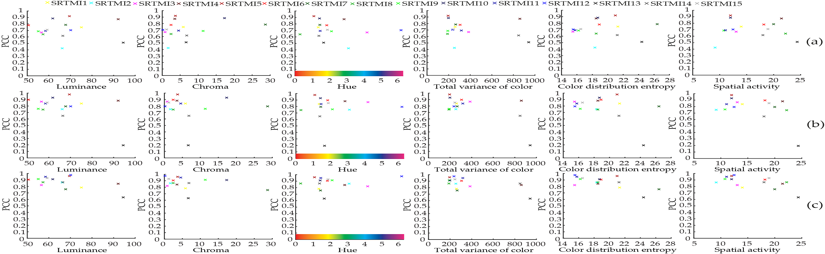
For SRTMI, plots of the content related features (x-axis) and the PCC performance (y-axis) of the three selected CD measures: (a) Δ E00 (b) Δ ECI and (c) Δ ECH.
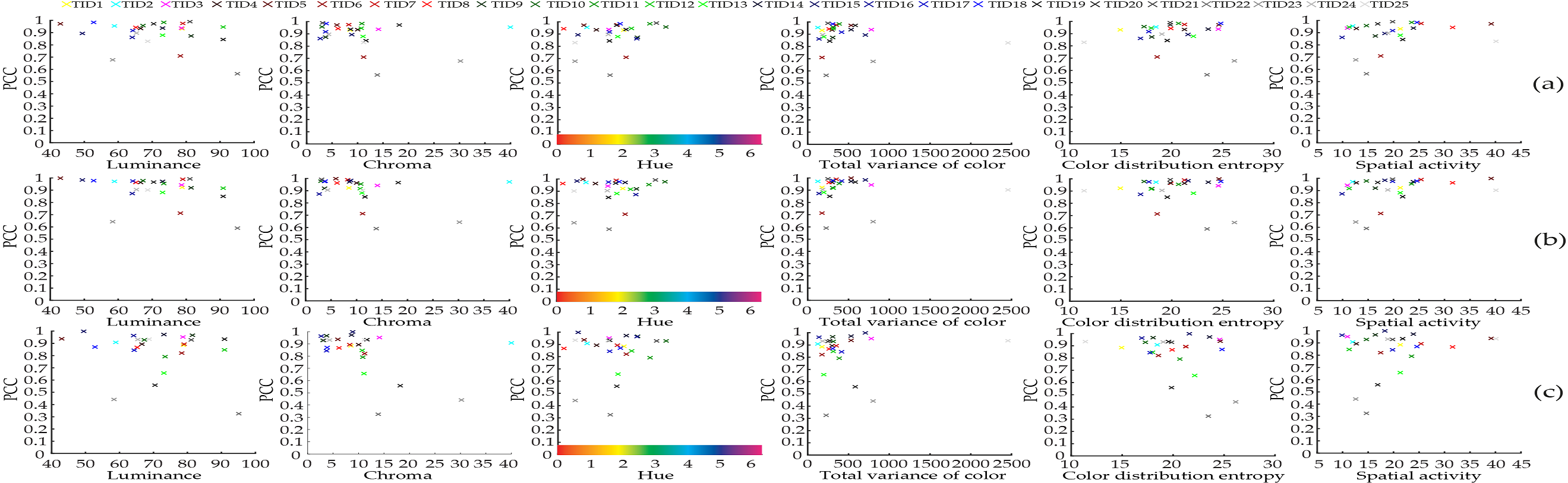
For mean shift subset from TID2013, plots of the content related features (x-axis) and the PCC performance (y-axis) of the three selected CD measures: (a) Δ E00 (b) Δ ECI and (c) Δ ECH.
The lowest performance for Δ E00, Δ ECI and Δ ECH is achieved on images SRTMI2 (for Δ E00 only) and SRTMI13. Image STRMI13 is the image with the highest spatial activity and color content (see Figure For SRTMI forth to sixth column) where the higher the spatial activity, the total variance of color or the color distribution entropy; the lower the performance, at least for our test images.
For mean shift subset from TID2013, we can conclude that the higher the chroma of the source image, the lower the performance of the CD measure. For instance, the performance achieved by Δ E00, Δ ECI and Δ ECH on images TID23, TID22 and TID20 is lower than 0.7 and their chroma values are higher compared with the other images. There are cases such as TID2 and TID20 where the color variation is low (only one color is covering most of the image) but the performance is high at least for Δ E00 and Δ ECI. That is, the performance of Δ ECH is more sensitive to high chroma values even under low color variance as the results on images TID2 and TID20 suggest. This is also reflected on Figure For mean shift subset from TID2013 (c) (fifth column) where the PCC decreases while the color distribution entropy increases. This agrees with the results of Habekost that the agreement of Δ E00 with human perception is lower on colors with a high chromatic component. From the spatial activity we can conclude that the performance of the CD measures is susceptible to the spatial activity changes in the source image (see Figure For mean shift subset from TID2013 sixth column). This is partially because the tested CD measures rely on global descriptive statistics from pixel-wise differences for computing the overall CD. In general, this kind of mechanism is very sensitive to the spatial activity because descriptive statistics are very sensitive to isolated outliers and isolated CDs are not well perceived by humans.
Conclusions and future work
Conclusions
We tested twenty state-of-the-art CD measures on selected data from three public databases
The CD measures were tested in images affected by CDs due to quantization noise, intensity shift, contrast change, change in color saturation and change in color balance
Quantization noise is one of less challenging types of color-related distortions where Δ E00, Δ ES 00, Ch, K∩, Δ EJ, Δ ECI, Δ ECH and Δ ED achieve a strong correlation with subjective scores
The tested CD measures perform well in the mean shift subset displaying a strong correlation with subjective scores: Δ E00, Δ ES 00, Δ EJ, Δ ECI, Δ ECH and Δ ED
Δ ECI and Δ ECH are the best performing measures on the distortion produced by color mapping achieving a strong correlation with human scores
The following CD measures are good candidates for assessing CDs on images affected by change of color saturation: Δ E00, Δ ES 00, Δ ECI, Δ ECH and Δ ED showing a strong correlation with subjective scores
In the contrast change subset none of the tested CD measures perform well
No statistically significant differences in terms of correlation were found when comparing Δ E00 and Δ ES 00 and Δ ED
The color content analysis suggests that the higher the color content of the source image the lower the performance of the CD measure
Relying on descriptive statistics from pixel-wise differences is very sensitive to the spatial activity of the image